Introduction
Welcome to this AI tutorial!
In this tutorial Artificial Intelligence (AI) topics are considered.
We continue with clustering (see Machine Learning tutorial using the expectation maximisation (EM) algorithm. This falls into the area of unsupervised probabilistic learning
Two more supervised-learning methods are considered: artificial neural networks (ANN) and support vector machines (SVM). Their accuracy will be compared to the linear regression model. Predictions and classifications minimise the error between given and predicted response.
Problem solving is achieved using optimisations. A brute-force approach and genetic algorithm (GA) will be introduced. Simulated annealing (SA) and exact methods are briefly mentioned.
A short introduction to Bayesian Belief Networks (BBN) will be given, which is commonly used when reasoning under uncertainty.
Probabilistic Learning - EM
We will use the iris dataset to identify three species. We assume the classification has not happen, hence, clustering is required.
Pairwise scatterplots show us the relationship of variables. This is usually the first step in an anlysis.
library(mclust)
clPairs(iris[,1:4])
There is another library GGally, which provides an even
more aesthetic visualisations.
library(GGally)
ggpairs(iris[,1:4])
The diagonal shows the density distribution of each feature. The upper-triangular matrix contains the Pearson-correlation coefficients. Here, wee see that petal length and sepal length are strongly correlated. Similarly, the petal’s length and width are strongly correlated.
Expectation maximisation
Expectation
maximisation (EM) is a probabilistic learning method. The algorithm
is used in the library mclust.
First we run the model with the default parameters. How many cluster have been identified?
# library(mclust)
em = Mclust( iris[,1:4], verbose = FALSE)
summary(em)
Answer: two with 50 and 100 nodes.
Now, we let the EM algorithm find three clusters using the
G variable. How well do the clusters agree with the defined
species.
em2 <- Mclust(iris[,1:4], G = 3, verbose = FALSE)
summary(em2)

table( em2$classification, iris$Species)
Answer: the first cluster agrees perfectly. The second and third have five flowers identified differently.
Learning - ANN & SVM
We will look at predicting eruptions. Please see the statistical learning tutorial for a gentle introduction.
General initialisations
We begin by defining two accuracy measures: root mean squared error
(RMSE) and mean absolute percentage error (MAPE). These will be used to
compare linear regression, ANN and SVM against each other. Our function
derr will display these measures.
#cat('\14'); rm(list=ls());graphics.off(); # for RStudio

rmse <- function(y,yh) {sqrt(mean((y-yh)^2))}
mape <- function(y,yh) {mean(abs((y-yh)/y))}
derr <- function(y,yh) {cat("MAPE:", mape(y, yh)*100,"%, RMSE:", rmse(y, yh))}
We need to do some general data pre-processing to evaluate the test-accuracy of the model.
We will use the faithful dataset (see Wikipedia for some
background information) and ?faithful for a data
description.
data(faithful); str(faithful)## 'data.frame': 272 obs. of 2 variables:
## $ eruptions: num 3.6 1.8 3.33 2.28 4.53 ...
## $ waiting : num 79 54 74 62 85 55 88 85 51 85 ...Your first task is to divide the data into train and
test data. Create sample indices for approximately 70% of
the faithful data used for training purposes. For
reproducibility initialise the random number generator with seed 7. We
will need the test-response repeatedly, hence, save it as \(y\). Show the first three records of
train, test and y.
n = nrow(faithful); ns = floor(.7*n);
set.seed(7); I = sample(1:n,ns);

train = faithful[I,]
test  = faithful[-I,]
y  = test$eruptions # will be used frequently
train[1:3,]; test[1:3,]; y[1:3]
Linear model (for comparisons)
We begin with a quick review of linear regression (see SL-LR for details).
flm = lm(eruptions ~ waiting, data = train)
yh = predict(flm, newdata = test) ### Test-accuracy
derr(y, yh)
The figure below visualises the eruption time (in minutes) for the predictions and observations over the waiting time (in minutes) for the entire data set.
ggplot(faithful, aes(waiting,eruptions)) + geom_point() +
  geom_point(data=data.frame(waiting = faithful$waiting,
    eruptions = predict(flm, newdata = faithful)), colour="purple")
The above graph reveals that there are apparently two types of erruption times. Short ones, which last about two minutes; and longe ones with about 4.4 minutes. furthermore, the graph reveals that waiting time must have been rounded, because many dots are “stacked up”.
Another typical visualisation is to plot predictions versus observations.
observations = faithful$eruptions;
predictions  = predict(flm, newdata = faithful)
qplot(observations, predictions)+geom_abline(slope = 1)
For an optimal model all points have to lay on the diagonal.
ANN model
We will create a neural network with one hidden layer that contains
three neurons. The ANN requires the library neuralnet.
Other interesting neural network libraries are: nnet,
gamlss and RSNNS.
Task, use the above neural network to predict the eruption times for 40, 60, 80 and 100 waiting-time.
library(neuralnet)

ann = neuralnet( eruptions ~ waiting,
           data = train,
           hidden = 3,
           linear.output = TRUE)
### Usage
predict(ann, data.frame(waiting=c(40, 60,80,100)))
That means iw we wait 80 minutes the expected eruption time will be 4.38 minutes.
what is the test-accuracy (MAPE, RMSE) for this model?
yh = predict(ann, newdata = test)
derr(y, yh)
That means, this ANN MAPE is approximately five percent better than the linear regression.
The ANN can be visualised using the common plot command.
(Note: only works in RStudio currently)
plot(ann)You will see the following graph:
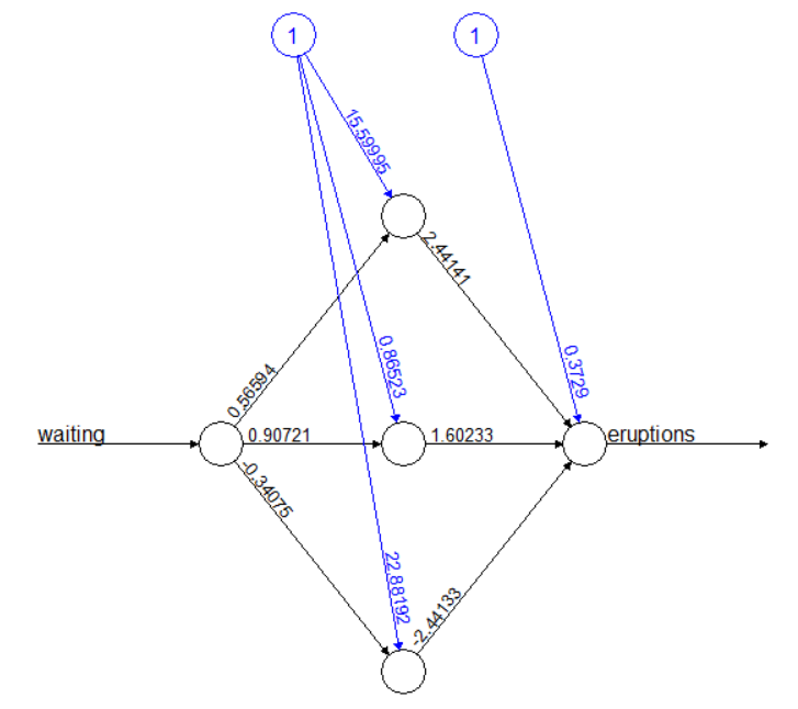
It shows the input layer (waiting - actually only one
neuron), the hidden layer with three neurons, and the output layer
(eruptions - just one neuron). The result of the output
layer is also known as hypothesis. The blue nodes are the
bias units.
For instance, assume the waiting time is \(a_{11}=2\) minutes. Hence, the first neuron
in the hidden layer \(a_{21}\) gets as
input \(15.6 + 0.566 a_{11} =
w_{10}a_{10}+w_{11}a_{11}\). Then the activation function
“fires”. By default neuralnet uses the logistic function as
activation function \(f\). This feeds
into the output neuron, which has the same activation function. Hence,
the eruption time is \(a_{31}=f(\sum_{i=1}^4
w_{2i}a_{2i})\).
The library NeuralNetTools allows another way to plot
ANNs using plotnet(ann). There
is a blog discussing visualisation of neural networks.
Again, the figure below visualises the eruption time (in minutes) for
the predictions and observations over the waiting time (in minutes) for
the entire data set. However, the neural network model ann
is used.
ggplot(faithful, aes(waiting,eruptions)) + geom_point() +
  geom_point(data=data.frame(waiting = faithful$waiting,
    eruptions = predict(ann, newdata = faithful)), colour="blue")
The figure seems to better fit the data. It goes through the middle of the two clusters.
The quality is illustrated with the following graph.
observations = faithful$eruptions;
predictions  = predict(ann, newdata = faithful)
qplot(observations, predictions)+geom_abline(slope = 1)
It can be seen that there is a systematic error at prediction time 2.0 and 4.4 minutes.
Support Vector Machines (SVM)
A support
vector machine model with default configuration is created. The
library e1071 is required.
sm = svm (eruptions ~ waiting, data = train)
yh = predict(sm, newdata = test)
### Usage
predict(sm, data.frame(waiting=c(40, 60,80,100)))yh = predict(sm, newdata = test)
derr(y, yh)We note that the test-accuracy is better than the one from the ANNs.
Visual the models predictions for the entire data set.
ggplot(faithful, aes(waiting,eruptions)) + geom_point() +
  geom_point(data=data.frame(waiting = faithful$waiting,
    eruptions = predict(sm, newdata = faithful)), colour="red")
Problem solving - GA & SA
Knapsack problem
A knapsack with a weight restriction \(\hat{w}\) has to be packed with items. Each item \(i\) has a weight and a value \(v_i\).
The objective is to maximise the total value by deciding whether to pack or not pack an item \(x_i\), i.e. \(x_i \in \lbrace 0,1\rbrace\)
\[ \max_{x} \lbrace\sum_{i=1}^n v_i x_i : \sum_{i=1}^n w_i x_i \leq \hat{w} \rbrace \]
By the way, this is the same as: \(\max_{x} \lbrace vx : wx \leq \hat{w} \rbrace\) in vector notation.
Let us assume \(v = \begin{bmatrix}6& 5& 8& 9& 6& 7& 3\end{bmatrix}\), \(w = \begin{bmatrix}2&3&6&7&5&9&4\end{bmatrix}\) and \(\hat{w} = 9\). What items should be packed?
We begin with defining the data.
v  = c(6, 5, 8, 9, 6, 7, 3) # values
w  = c(2, 3, 6, 7, 5, 9, 4) # weights
wh = 9 # weight limit (including values)
n  = length(v) # number of elements (required later)
Warmup
Let \(x\) be decision vector, which
items have to be packed. Define x such that item 1 and 3
are packed. What is the value and weight of packing item 1 and 3 use the
dot-product.
x = c(1,0,1,0,0,0,0)
v %*% x # value
w %*% x # weight
Brute Force
Write a function that finds the optimal solution using a brute force approach. That means all configurations (here, packing options) are tested, and all feasible solutions are evaluated (Note: you may want to do a few preparation exercises first - see below).
# Brute force (maximise value)
knapsackBF <- function(v, w, wh) {
  n = length(v); best.v = -Inf;
  for (nb in (0:2^7-1)) {
    x = as.integer( intToBits(nb) )[1:n]
    if (w %*% x <= wh) { # then weight constraint ok
      if (v %*% x > best.v) { # then new best value
        best.v = v %*% x
        sol = x
        cat('New solution:', x,">> value:", best.v,"\n")
      }
    }
  }
  cat("Best solution value:", best.v, "\nusing x = ", sol, "\n")
  return (sol)
}
x = knapsackBF(v, w, wh)
That means item 1 and 4 need to be packed (use
which(x==1)). These items have a value of 15 =
v %*% x (individual values are 6 and 9 =
v[sol==1]) with weights 2 and 7.
Practice (preparational exercises)
Convert the number 6 into bits using intToBits() and
convert the bits back into integers.
bits = intToBits(6)
as.integer(bits)
Genetic Algorithm
We will use a Genetic Algorithm with binary chromosome algorithm
(rbga.bin) to solve the above Knapsack problem. The
algorithm is part of the genalg library.
The algorithm requires an evaluation function, which contains the
constraints and objective function. Note that rbga.bin only
minimises, i.e. we need to invert the objective to maximise.
Your task is to write the evaluation function evalFun
for the Knapsack problem. Assume that \(v\), \(w\)
and \(\hat{w}\) are known in the global
environment; and \(x\) is the input.
Return \(-v\cdot x\) if the weight is
less than \(\hat{w}\), otherwise \(+\infty\). Test the function with \(x =
\begin{bmatrix}1&1&0&0&0&0&0\end{bmatrix}\).
Is the solution feasible? If yes, what is the solution value?
evalFun <- function(x) {
  if (w %*% x <= wh) { # then weight constraint ok
    return ( -(v %*% x) ) # invert value to maximise
  } else { return(+Inf)}
}

evalFun(c(1,1,0,0,0,0,0)) # test
Answer: The solution is feasible and the solution value is -11.
Now let us call the GA using most of the default parameter settings. What is the best solution and its value?
myGA <- rbga.bin(evalFunc = evalFun, size = n)

# Best solution
best.v = -min(myGA$best) # best found solution value in each iteration
idx = which.min(myGA$evaluations) # index of individual with best value
sol = myGA$population[idx,]  # best found solution

cat("Best solution value:", best.v, "\nusing x = ", sol, "\n")
Answer: the best found solution (in this case it is also the best solution) is \(x = \begin{bmatrix}1&0&0&1&0&0&0\end{bmatrix}\) with solution value 15.
What default parameters are shown using the summary
function on myGA?
cat(summary(myGA))Answer: population size, number of generations, elitism and mutation chance.
Change the mutation chance (mutationChance) to \(\frac{1}{n}\), population size
(popSize) to 20 and the number of iterations
(iters) to 40.
Did the algorithm still return the same solution? Did the algorithm find the solution faster?
myGA <- rbga.bin(evalFunc = evalFun, size = n, mutationChance = 1/n, popSize = 20, iters = 40)

best.v = -min(myGA$best); sol = myGA$population[which.min(myGA$evaluations),]
cat("Best solution value:", best.v, "\nusing x = ", sol, "\n")
Answer: the same solution was found and the algorithm ran faster. Note: results may vary because of different random number generation.
Simulated Annealing
Simulated Annealing is a meta-heuristic used for optimisation problems. Please explore TSP blog and related Github repository.
Exact Approaches
The MathProg Solver on Smartana.org includes several examples to get you started with formulating optimisation problems.
Please see: Examples >> Basic Optimisations >> Knapsack to find the mathematical program to solve the Knapsack problem exactly.
Games - minimax
We will implement the minimax algorithm and integrate \(\alpha\)-\(\beta\) pruning into it.
Our objective is to create a simple example to test our implementation of the minimax algorithm. We assume a simplified chess game. White has two options to make a move. Similarly, black has two options to respond. At a game-tree depth three all positions are evaluated. The figure below shows the minimax example, we’d like to reproduce.
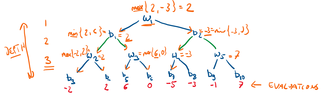
Each node name in this example represents a position (state).
Functions for the positions, node evaluations and game-over state are hard-coded, but can be easily replaced for other games.
getPositions <- function(pos){
  switch (pos,
          'w1'=c('b1','b2'),   'b1'= c('w2','w3' ),
          'b2'= c('w4','w5' ), 'w2'= c('b3','b4' ),
          'w3'= c('b5','b6' ), 'w4'= c('b7','b8' ),
          'w5'= c('b9','b10'))
}
cat("Positions resulting from b1:", getPositions('b1'), "\n") # test

gameOver <- function (pos) {
  return(FALSE) # always returns FALSE (template code)
}

evaluate <- function(pos) {
  switch(pos,
         'b3' = -2, 'b4' =  2, 'b5' =  6, 'b6' =  0,
         'b7' = -5, 'b8' = -3, 'b9' = -1, 'b10'=  7)
}
cat("Value of position b3 is ", evaluate('b3'), "\n") # test
Next we will implement the minimax algorithm.
minimax <- function(pos='w1', depth = 1, player = TRUE){
  if (depth == 0 || gameOver(pos)) {
    return (evaluate (pos))
  }
  if (player) {
    eval.max = -Inf;
    for (p in getPositions(pos)){
      eval.p = minimax(p, depth-1, FALSE)
      eval.max = max(eval.max, eval.p)
    }
    return (eval.max)
  } else {
    eval.min = +Inf;
    for (p in getPositions(pos)){
      eval.p = minimax(p, depth-1, TRUE)
      eval.min = min(eval.min, eval.p)
    }
    return (eval.min)
  }
}
cat("Postion evaluation (depth 3):", minimax(depth = 3),"\n") ### Test function\(\alpha\)-\(\beta\) pruning
minimaxab <- function(pos='w1', depth = 1, player = TRUE,
                      alpha = -Inf, beta = +Inf){
  if (depth == 0 || gameOver(pos)) { return (evaluate (pos))}
  if (player) {
    eval.max = -Inf;
    for (p in getPositions(pos)){
      eval.p = minimaxab(p, depth-1, FALSE, alpha, beta)
      eval.max = max(eval.max, eval.p)
      alpha = max(alpha, eval.p)
      if (beta <= alpha) {break}
    }
    return (eval.max)
  } else {
    eval.min = +Inf;
    for (p in getPositions(pos)){
      eval.p = minimaxab(p, depth-1, TRUE, alpha, beta)
      eval.min = min(eval.min, eval.p)
    }
    beta = min( beta, eval.p)
    if (beta <= alpha) {break}
    return (eval.min)
  }
}
minimaxab(depth = 3, alpha = -Inf, beta = +Inf) ### Test function
Chess
In the previous section we indicated how to write an algorithm which finds the best chess move given an appropriate evaluation function.
The library rchess has the class
Chess, which contains several useful methods (names(chess))
such as plot (display board), pgn (notation)
and in-check.
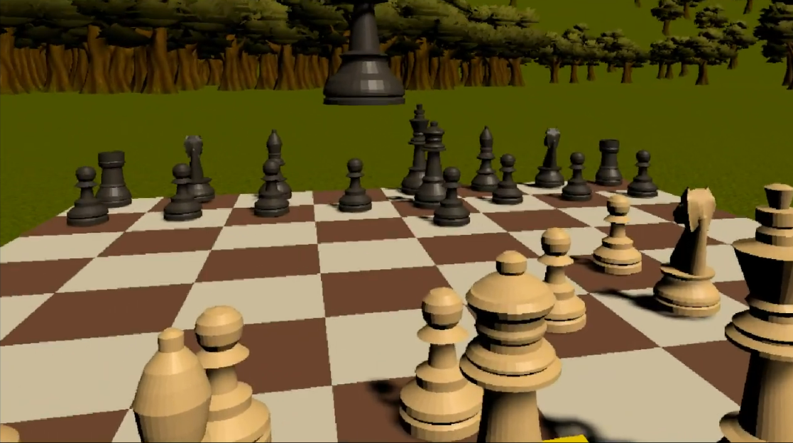
Let us begin with white’s move (first ply).
library(rchess)
chess <- Chess$new()
chess$move("e4")
plot(chess)
Let us do a few more moves.
chess$move("c5") # Black's move
chess$move("Nf3")$move("e6")
chess$move("Na3")$move("Nc6")
chess$move("Nc4")$move("Nf6")
chess$move("Nce5")  # how to select from two figures
plot(chess)
Now, we could use our minimax algorithm if we had an
evaluation function. A simple evaluation function is to count the
material. chess$get() returns the colour and figure type.
However, we will immediately jump to one (if not the) most popular chess
engine in the world Stockfish.
We will replicate the above moves in Stockfish, and let Stockfish find a move.
library(stockfish)
engine <- fish$new()
engine$uci()
engine$isready() # should return true
moves = "moves e2e4 c7c5 g1f3 e7e6 b1a3 b8c6 a3c4 g8f6 c4e5"
engine$position(type="startpos", position=moves)
response = engine$go()
engine$quit()
response
That means the chess engine is ready to receive our moves. It finds black’s move Nxe4 and anticipates white’s next move Nxc6.
Let me introduce a simple “initial” function (getPly,
i.e. it needs a bit more work) that converts between rchess
and stockfish notation. This allows us to plot Stockfish’s
response.
library(tidyverse)
getPly <- function(response){
  ply  = str_split(response, " ")[[1]][2]
  from = substr(ply,1,2); to = substr(ply,3,4);
  fig  = toupper(chess$get(from)$type)
  if (fig == 'P') fig = "";
  hit  = !is.null(chess$get(to)$type)
  if (hit) {mv=paste0(fig,'x',to)} else {mv=paste0(fig,to)}
  return(mv)
}

mv = getPly(response)
chess$move(mv)
plot(chess)
The above code linked with an interactive board returns an almost unbeatable chess programme. Stockfish uses the Universal Chess Interface, which enables it to communicate with any user interface. Please find Stockfish’s source code on GitHub, which includes more details about the UCI options available and the source code. The source code reveals the evaluation function, and how the best move is found.
Tic-Tac-Toe
Please explore this Tic-Tac-Toe blog.
Practice makes perfect
Write a recursive function that computes factorial powers
facPow for positive integers. (Note this function exists as
factorial.) Test the function for \(n=5\).
\[ n! = n (n-1)!, ~ 0!=1, n>1 \]
facPow <- function(n){
  if (n==0) return(1) else return ( n * facPow (n-1) )
}
facPow (5)
Next implement the Fibonacci numbers as recursive function (see previous loop tutorial).
Reasoning under Uncertainty - BBN
Reasoning under Uncertainty with Bayesian Belief Networks (BBN).
An interactive environment can be found using the library
BayesianNetwork and the function
BayesianNetwork().
The tutorial is based on an example from the bnlearn.com site.
Here, is a quick data description (Ness (2019)):
- Age (A): It is recorded as young (young) for individuals below 30 years, adult (adult) for individuals between 30 and 60 years old, and old (old) for people older than 60.
- Sex (S): The biological sex of individual, recorded as male (M) or female (F).
- Education (E): The highest level of education or training completed by the individual, recorded either high school (high) or university degree (uni).
- Occupation (O): It is recorded as an employee (emp) or a self employed (self) worker.
- Residence (R): The size of the city the individual lives in, recorded as small (small) or big (big).
- Travel (T): The means of transport favoured by the individual, recorded as car (car), train (train) or other (other)
Defining the network
#library(bnlearn)
dag <- empty.graph(nodes = c("A","S","E","O","R","T"))
arc.set <- matrix(c("A", "E",
                    "S", "E",
                    "E", "O",
                    "E", "R",
                    "O", "T",
                    "R", "T"),
                  byrow = TRUE, ncol = 2,
                  dimnames = list(NULL, c("from", "to")))
arcs(dag) <- arc.set
# nodes(dag)
plot(dag)
States and Probabilities
We defined the states and probabilities and display all conditional probability tables (CPTs).
A.lv <- c("young", "adult", "old")
S.lv <- c("M", "F")
E.lv <- c("high", "uni")
O.lv <- c("emp", "self")
R.lv <- c("small", "big")
T.lv <- c("car", "train", "other")

A.prob <- array(c(0.3,0.5,0.2), dim = 3, dimnames = list(A = A.lv))
S.prob <- array(c(0.6,0.4), dim = 2, dimnames = list(S = S.lv))
E.prob <- array(c(0.75,0.25,0.72,0.28,0.88,0.12,0.64,0.36,0.70,0.30,0.90,0.10),
                dim = c(2,3,2), dimnames = list(E = E.lv, A = A.lv, S = S.lv))
O.prob <- array(c(0.96,0.04,0.92,0.08), dim = c(2,2),
                dimnames = list(O = O.lv, E = E.lv))
R.prob <- array(c(0.25,0.75,0.2,0.8), dim = c(2,2),
                dimnames = list(R = R.lv, E = E.lv))
T.prob <- array(c(0.48,0.42,0.10,0.56,0.36,0.08,0.58,0.24,0.18,0.70,0.21,0.09),
                dim = c(3,2,2), dimnames = list(T = T.lv, O = O.lv, R = R.lv))
cpt <- list(A = A.prob, S = S.prob, E = E.prob, O = O.prob, R = R.prob, T = T.prob)
cpt
Applying the BBN
survey = custom.fit(dag, cpt)
#rbn(survey, n = 10)
newdata = data.frame(A = factor("young", levels = A.lv),
                    S = factor("F", levels = S.lv),
                    E = factor("uni", levels = E.lv),
                    O = factor("self", levels = O.lv),
                    R = factor("big", levels = R.lv))

predict(survey, node = "T", data = newdata)
cpquery(survey, event = (S == "M") & (T == "car"), evidence = (E == "high"))Resources
- An excellent introduction to learning methods is James et al. (2013). This book can also be found online.
- A classic introduction into the field of AI is Russell and Norvig (2020) book.
Acknowledgment
This tutorial was created using RStudio, R, rmarkdown, and many other
tools and libraries. The packages learnr and
gradethis were particularly useful. I’m very grateful to Prof. Andy
Field for sharing his disovr package,
which allowed me to improve the style of this tutorial and get more
familiar with learnr. Allison Horst wrote a very
instructive blog “Teach
R with learnr: a powerful tool for remote teaching”, which
encouraged me to continue with learnr. By the way, I find
her statistic
illustrations amazing.
References