Introduction
Welcome to this Statistical Learning tutorial.

In this tutorial linear regression will be applied to predict the eruption duration of a geyser.
Logistic regression will be used to predict whether an eruption of a geyser is long or short. Another case study is given to show some more aspects of classifications.
The overall aim is to introduce supervised learning, i.e. both input and output are known and allow the learning of a model. Another aim is to review fundamentals of statistics, such as sample standard deviation, correlation, covariance, and others. The objectives are:
- To recognise the benefit of correlation;
- To distinguish between confidence and prediction interval;
- To split data into training and test data;
- To understand and apply linear and logistic regression to challenges;
- To know the difference between prediction and classification;
- To quantify the goodness/quality/accuracy of a model.
The major learning outcome is to gain familiarity with the data science language .
Please be sure you have done the datatypes tutorial and controls & functions tutorial.
Linear Regression
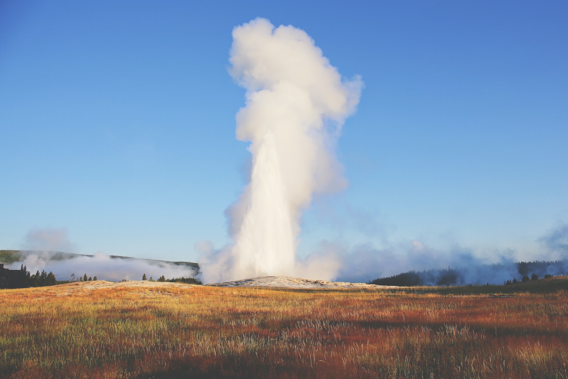
Old Faithful is a geyser in Yellowstone National Park in Wyoming, United States. Assume you have waited 80 minutes. How long will the eruption last? Such questions we would like to answer. Generally, we would like to derive a model that predicts the duration of the geyser’s eruption, depending on how long you had to wait.
We will begin with an exploration of the data. This is followed by deriving a linear regression model for predictions. Then the quality of the model is discussed. Finally, the confidence and prediction intervals are introduced, so, that we can explain the certainty and range of the expected eruption time.
Exploring data
We will explore the structure and the first few records (i.e. rows) of the data. Some basic descriptive statistics for each feature (i.e. column) will be looked at. The above gives us a basic understanding of the data.
Structure, Preview and Statistics
Three methods give initial insights about the data:
strshows the structure of the data;headprovides a preview the first rows of the data set;summarygives a list of basic descriptive statistics.
How many observations and variables are in the “faithful” data set?
str (faithful)Answer: 272 observations and 2 variables
Display the first six observations?
head (faithful)Answer: 3.6 79, …
What is the shortest, expected and third quartile eruption duration?
summary(faithful)Answer: Min 1.6min, mean: 3.488 and 3rd Quartile is 4.454min.
Visual inspection
Display the data as a scatter plot and add a “trend line”.
# library(ggplot2)
g <- ggplot(data = faithful,aes(waiting,eruptions))+
   geom_point()+stat_smooth(method="lm")
g
The data seems to have some linear relationship. Although it looks like there are two classes, one with long durations (above 3min) and another one with short durations (below 3min) - more about this in the logistic regression section.
Let us have a bit of fun: plot the means, min and max, etc. and add some colour and size. Let us also add the unit to the x and y axes.
# library(ggplot2)
attach(faithful)
me = mean(eruptions); sde=sd(eruptions);
g +  geom_hline(yintercept=me) +
     geom_text(aes(x=50, y=me, label=sprintf('y=%.2f',me), vjust=-0.4))+
     geom_vline(xintercept=mean(waiting)) +
     geom_hline(yintercept=min(eruptions), color="red", size=2)+
     geom_hline(yintercept=max(eruptions), color="blue", size=2)+
     geom_hline(yintercept=me+sde, color="red", linetype=4)+
     geom_hline(yintercept=me-sde, color="red", linetype=4)+
     xlab('x = waiting time [minutes]')+
     ylab('y = eruptions [minutes]')
Correlation
We can also see that the data is correlated:
cor(faithful) gives us 0.901. That means the Pearson
Correlation Coefficient (PCC) \(r\) reveals a strong association between
the variables. The PCC is defined as: \[ r =
r_{X,Y} = \frac{s_{XY}}{s_X s_Y},\] where \(s_X\) is the sample standard deviation of
\(X\) and \(s_{XY} = \text{cov}(X,Y)\) is the sample
covariance. The sample standard deviation \(s\) is obtained form the sample variance
\(s^2\) by taking the square root and
is defined as: \[s^2 = \frac{1}{n-1}
\sum_{i=1}^n (x_i-\bar{x})^2.\] The sample covariance is defined
as: \[
\text{cov}(x,y) = \frac{\sum_i(x_i-\bar{x})(y_i-\bar{y})}{n-1}.
\]
The above can be determined with the following functions in
:
correlation cor(), standard deviation sd,
variance var() and covariance cov().
Verify that the functions are correct. You can use the
attach function for easier access of a
data.frame.
attach(faithful)
x = eruptions; y = waiting; n = nrow(faithful);
cat('cor(x,y) = ',  cor(x,y),
    '=cov(x,y)/(sd(x)*sd(y)) =', cov(x,y)/(sd(x)*sd(y)))
cat('cov(x,y) = ',  cov(x,y),
    ' = ', sum( (x - mean(x)) * (y - mean(y)) )/(n-1))
For simple linear regression the squared PCC is equivalent to the coefficient of determination, i.e. \(r^2 = R^2\). Note, that this is not generally true.
The coefficient of determination is defined as: \[ R^2 = \frac{\sum_{i=1}^n (\hat{y}_i - \bar{y})^2}{\sum_{i=1}^n (y_i - \bar{y})^2}\] That means, that even without the prediction model we are already in the position to give an accuracy statement about the goodness of the model. The coefficient of determination is 0.81.
Prediction Model
Next we will develop a linear regression prediction model, and answer the question: What are the coefficients of the model \(\hat{y}= \beta_0+\beta_1 x\)?
formula =  eruptions ~ waiting #symbolic description of model
model   = lm(formula, data=faithful) # fit a linear model

c = model$coefficients # coefficients(model) #an alternative
c
Solution: \(\beta_0\) = -1.874 and \(\beta_1\)=0.0756
Let us approach this a bit more formally.
A real-world model \(f\) (systematic information) is explained by: \[y=f(X)+\epsilon,\] where \(y\) is the output (response, observed values), \(X = (x_1, \cdots, x_p)\) is the input (known also as predictors, variables, features) and \(\epsilon\) is the random error. All inputs and outputs are real with \(X \in \mathbb{R}^{n\times p}\) and \(y \in \mathbb{R}^{n}\). Here, \(n\) is the number of observations and \(p\) is the number of features.
A prediction model \(\hat{f}\) (estimate for \(f\)) generates predictions \(\hat{y} \in \mathbb{R}^{n\times 1}\) using existing (real) input \(X=\begin{bmatrix}X_i\end{bmatrix}=\begin{bmatrix}x_j\end{bmatrix}\) (rows \(X_i\), columns \(x_j\)): \[\hat{y}=\hat{f}(X).\] Using the multivariate linear regression model the prediction model becomes: \[\hat{y}=\hat{f}(X) = Xb,\] where \(b \in \mathbb{R}^{1\times p}\) is a row-vector.
Note: that one of the features of \(X\) is a one-vector (i.e. all elements are ones).
The method lm computes \(b\) by minimising the mean squared error:
\[\text{MSE}=\frac{1}{n}
{\sum_{i=1}^{n}\left(y_{i}-\hat{y}_i\right)^{2}}.\]
Using the Model
In the previous section we determined the models coefficient’s and
saved them as vector c.
What is the eruption duration given that we waited \(w=80\) minutes? Hint: Use the coefficients from before.
w = 80 #min waiting time
d = c[1] + c[2]*w
d
Solution: We expect to observe an eruption lasting for 4.18min (given 80min waiting time).
As you can see in the result the name of c[1] was used
to name the variable d. You can change this using
names().
names(d) <- 'duration'
d
Multiple predictions: Predict the eruption times for times 40, 60, 80 and 100 minutes. Can you observe any systematic change?
p = data.frame(waiting=c(40, 60,80,100))
predict(model,p)
Answer: every 20 minutes of waiting gives us an additional 1.51
minutes of eruption (see waiting coefficient \(\beta_1\)).
Math Approach(optional)
Here, we will show to approaches to determine the model analytically. Note, this section is optional. It assumes some familiarity with linear algebra (vectors, matrices, calculus).
Our objective is to minimise the error vector \(\epsilon\) between the vectors \(y\) (observed values) and \(\hat{y}\) (modelled values), because \(y = \hat{y} + \epsilon\). If you look at a 2D-vector it is obvious that the error is at a minimum, when \(\hat{y}\) and \(\epsilon\) are orthogonal, i.e. \(\hat{y} \bot \epsilon\). Two vectors are orthogonal when their product is zero: \[ \hat{y} \bot \epsilon \Rightarrow\hat{y}^\intercal \epsilon=0.\]
The modelled (predicted) values are determined by \(\hat{y}=Xb\). The error is \(\epsilon = y - \hat{y} = y - Xb\). Using the above two formulas allows us to substitute \(\hat{y}\) and \(\epsilon\): \[ \hat{y}^\intercal \epsilon=0 \Rightarrow(Xb)^\intercal (y-Xb)=0.\] Applying the transposition, associative law, distributive law, and realising that we can drop \(b^\intercal\) gives us: \[ (Xb)^\intercal (y-Xb) = b^\intercal X^\intercal (y-Xb) = 0 \Rightarrow X^\intercal y = (X^\intercal X)b \] Since, \(X^\intercal X\) is a squared matrix we can compute the inverse. \[ X^\intercal y = (X^\intercal X)b \Rightarrow(X^\intercal X)^{-1}X^\intercal y = (X^\intercal X)^{-1}(X^\intercal X)b\] Hence, the prediction model coefficients are: \[ b = (X^\intercal X)^{-1}X^\intercal y \]
Now let us use the above formula to derive the coefficients for the
geyser prediction model. The interesting aspect is that the matrix
inverse is obtained using solve rather than
^(-1).
y = faithful$eruptions
x = faithful$waiting
e = rep(1,nrow(faithful)) # one vector
X = cbind(e,x)

b = solve((t(X)%*%X)) %*% t(X) %*% y
b
Note that sometimes there are duplicated records, which may exist on purpose (e.g. same scenario observed multiple times). In this case the pseudo-inverse (generalised-inverse) needs to be used, e.g. the Moore-Penrose inverse.
library(MASS) # obtain ginv function

bp = ginv((t(X)%*%X)) %*% t(X) %*% y
bp
Goodness/Quality of Model
How much of the total variation can be explained by the model?
summary(model)$r.squaredAnswer: 81.1% can be explained.
What is the MSE? Write a function that implements:
\[\text{MSE}=\frac{1}{n} {\sum_{i=1}^{n}\left(y_{i}-\hat{y}_i\right)^{2}},\]
and determine the MSE for all observed and modelled values.
yh = predict(model)
y  = faithful$eruptions

mse  <- function(y,yh) {mean((y-yh)^2)}
mse(y,yh)
Determine the RMSE, use the function implemented previously.
\[\text{RMSE}=\sqrt{\text{MSE}}=\sqrt{\frac{1}{n} {\sum_{i=1}^{n}\left(y_{i}-\hat{y}_i\right)^{2}}}\]
sqrt(mse(y,yh))Note: The RMSE is commonly used to describe the accuracy of the model.
Training and Test Data
It is common to divide the data into training and test data. This gives reassurance that the fitted model will work for unseen data (simulated by the test data). The training data is used to train and learn the model. The test data ‘’validates’’ the learned model.
Let us do a 70:30 data split, i.e. 70% of the data will be used for
learning the model randomly; and the remaining 30% of the data will be
used to test the accuracy of the model. We will make the split
reproducible by fixing the seed of the random number with
set.seed(1).
n = nrow(faithful)  # number of observations
ns = floor(.7*n)    # 70% times n = number of training data records
set.seed(1)         # seed of random generator (for reproducibility)
I = sample(1:n, ns) # sample of indexes
train = faithful[I,]    # training data (=70% of data)
test  = faithful[-I,]   # test data (=30% of data)
Use the training data to learn the linear regression model, and provide the RMSE for the training data.
lr <- lm (eruptions ~ waiting, data=train)

yh = predict(lr)
y  = train$eruptions
rmse  <- function(y,yh) {sqrt(mean((y-yh)^2))}
rmse(y,yh)
Now compute the test RMSE for the model to see how well it performs for unseen data.
yh = predict(lr, newdata = test)
y  = test$eruptions
rmse(y,yh)
You should observe that the RMSE for the test data is higher than the RMSE for the training data.
Note a different seed will lead to a different accuracy. Hence, it would be better to repeat the splitting multiple times and use the average accuracy instead.
Confidence Interval
Determine the expected eruption time using many independent samples of 80 min of waiting. What is our 95% confidence interval of the expected eruption duration?
attach(faithful)     # attach the data frame
my.lm = lm(eruptions ~ waiting)
w = data.frame(waiting=80)
predict(my.lm, w, interval = "confidence")
Answer: The CI of the expected eruption time is [4.105, 4.248]
Prediction Interval
Which eruption time will we observe with 95% certainty when the waiting time for the eruption was 80 minutes?
predict(my.lm, w, interval = "predict")Answer: we will observe an eruption time which is between 3.2min and 5.2min.
Overall we expect the eruption to last for 4.18 minutes (with a 95% - CI of [4.105, 4.248]) given a 80 minutes waiting time. We predict that the eruption will last between 3.2min and 5.2min with 95% certainty, when the eruption occurs after 80 minutes of waiting.
Practice makes perfect
Use the code written previously to specify the training and test data by embedding it in a function and show its usage.
dataSplit <- function(data=faithful, p=.7, seed=1){
  n = nrow(data) # number of observations
  ns = floor(p*n) # 70% times n = number of training data records
  set.seed(seed) # seed of random generator (for reproducibility)
  I = sample(1:n, ns) # sample of indexes
  train = data[I,] # training data (=70% of data)
  test = data[-I,] # test data (=30% of data)
  D = list(train=train, test=test)
  return(D)
}

D = dataSplit()
str(D)
# attach(D) # to have access to train and test directly
Analyse the intercountry life-cycle savings data.
- Provide basic descriptive statistics (what is the expected personal saving?);
- Analyse the correlations (which two features have the highest correlation?);
- What is the root mean squared error of the LR model?
- What are the aggregated personal savings for pop15=35, pop75=2.3, dpi=800, ddpi=3.5? (use linear regression)
summary(LifeCycleSavings)
r = cor(LifeCycleSavings)
r[r==1]=0; max(r)

lr <- lm(sr ~ ., data = LifeCycleSavings)

yh = predict(lr)
y  = LifeCycleSavings$sr
sqrt(mean(sum((y-yh)^2))) # RMSE

df <- data.frame(pop15=35, pop75=2.3, dpi=800, ddpi=3.5)
predict(lr, newdata=df)
Answer: (a) mean sr = 10.51, (b) pop75 and dpi, (c) RMSE = 25.1, (d) sr = 9.70
Logistic Regression
Faithful example
Create a new feature long_eruptions for the faithful
dataset. Set long_eruptions to one if the eruption duration
is more than three minutes and zero otherwise.
data("faithful")
faithful$long_eruptions = (faithful$eruptions>3)*1
str(faithful)
Visualise the two classes.
library(ggplot2)
ggplot(aes(x=waiting, y=eruptions,
           colour=factor(long_eruptions)),,
           data = faithful)+
  geom_point(show.legend = FALSE, size=2)
Divide the data into training and test data using a 70:30 split.
n = nrow(faithful); ns = floor(.7*n);
set.seed(7); I = sample(1:n, ns);
train = faithful[I,];test = faithful[-I,];
str(train); str(test)
Display the training and test data.
g1 <- ggplot(aes(x=waiting, y=eruptions, colour=long_eruptions),data = train)+
  geom_point(show.legend = FALSE)
g2 <- ggplot(aes(x=waiting, y=eruptions, colour=long_eruptions),data = test)+
  geom_point(show.legend = FALSE)

library(gridExtra)
grid.arrange(g1, g2, ncol=2)
Train the model using logistic regression.
logreg <- glm(long_eruptions ~ waiting, data = train, family = binomial )
logreg
Predict the classes for the test data.
p  = predict(logreg, newdata = test, type = "response")
yh = (p>.5)*1
cat('p=',p[1:8])
cat('yh=',yh[1:8])
Determine the accuracy of the model.
y  = test$long_eruptions
mean(y==yh)
Create a confusion matrix.
y  = test$long_eruptions
table(yh,y)
Do the above exercises again, but change the threshold of
long_eruptions to two minutes.
Case Study - Titanic

The ship - RMS Titanic - sank in the early morning hours of 15 April 1912 in the North Atlantic Ocean. The disaster led to significant changes in maritime regulations.
Develop a prediction model that checks whether a passenger would have survived based on his profile.
Data source
The data is obtained using the Titanic library. This is based on the
Kaggle data set. Check
the content of the titanic library. Does it contain a
training and test data set?
# library(titanic)
ls("package:titanic")
Please inspect the training and test data set. Does the test data set contain passenger information?
#?titanic_train
?titanic_test
Answer: no passenger information is available, i.e. we cannot determine the test accuracy of the model. Note: the information was not provided, since it is a competition on Kaggle.
By default there is another data set about the Titanic in the R environment. However, it contains only aggregated information.
There is a Titanic website, which contains even more data about the disaster.
However, we will use the previous train data set, and we will assume that this is the entire data available.
Explore data
Similar, to the linear regression explore the data using
names, head and summary.
- Does the data contain a
SurvivedandSexfield? - What is the name in the sixth record?
- How many records does the data set contain?
- How many elements are not available in the
Agefield?
T = titanic_train # assume from now on this is training and test data.
names(T)
head(T)
summary(T)
Answers: 1) yes; 2) James Moran; 3) 891; 4) 177.
Data cleaning
The field Age has several “not available(na)” entries.
Your task is to set those to the average age. What is the average
age?
# sum(is.na(T$Age))
mv = mean(T$Age, na.rm = TRUE)
T$Age[is.na(T$Age)] = mv
mv
Answer: 29.7 years.
Create a training set D that contains 80% of the data
(round down). How many records has D?
n = length(T$PassengerId) # number of passengers
ns = floor(0.8*n) # #records for training data set

set.seed(1) # fix random number generator
I = sample(1:n, ns) # create sample indizis (no repetitions)

I[1:10] # show the first 10 records
length(I); # or a bit more precise: length(unique(I))
D = T[I,]
Answer: 712.
Two models
Let’s derive two simple prediction models.
Model 1 - everyone dies
How many passengers have survived (died)? What is the corresponding percentage?
# library(dplyr)
aD <- D %>% group_by(Survived) %>% summarise(nb = length(PassengerId))
aD %>% mutate(pnb = nb/ns)
Answer: 278 survived (61.0%), 434 died (39.0%).
That means, if we assume everyone will die the model is correct 61% of the time for the training data.
Hence, let model 1 assume that everyone dies (=0). What is the accuracy for the test data?
test = T$Survived[-I]
mean(0 == test)
The above shows that model 1 is 64.2% correct for the test data. This is better than a random guess.
Model 2 - females survive
Let us inspect whether the gender has any impact.
aD2 <- D %>% group_by(Survived, Sex) %>% summarise(nb = length(PassengerId))
# aD2
# library (tidyr) # reshape aD2
aD2 %>% pivot_wider(Sex, names_from = Survived, values_from=nb)
The above table states: if your are female you are more likely to survive. What is test-accuracy for a model where all females survive?
pm <- rep(0,length(test)) # no one survives (as model 1)
pm[T$Sex[-I] =="female"]=1 # all females survive
mean(pm == test)
Answer: There is a 81% test-accuracy.
Logistic Regression Model
Let’s derive a logistic regression model. Previously, we found the existing field names.
names(D)From the previous models we have learned that Sex is an
important feature. Let us use this field to build the logistic
regression model f.
First model: Survived ~ Sex
f <- glm(Survived ~ Sex, data = D, family = binomial ) # would result in the same result as above
#f <- glm(Survived ~ Sex + Age + Pclass+ SibSp + Fare + Embarked, data = D, family = binomial )
#summary(f)
summary(f)$coef
Predict the probability for f and display the first 10
probabilities.
f_prob = predict(f, type = "response")
f_prob[1:10]
Transform the probabilities to the response variable. What threshold is used? Display the first five elements of \(\hat{y}\).
yh = rep(0, length(f_prob))
yh[f_prob>=0.5] = 1
yh[1:5]
Answer: 0.5
Confusion matrix
Build a matrix that shows the values predicted correctly and wrongly. What are the true positives (survivors identified correctly by the prediction model)? What are the true negatives (passengers that did not survive predicted correctly)?
C = table(yh, D$Survived)
C
Answer: The number of true positives is 192, and the number of true negatives is 364.
What is the train-accuracy of this model?
# correctly predicted in training set
C[1,1]+C[2,2] # true negatives + true positives
# cat( 'ns = ', ns, ' = ', length(D$Survived), ' = ', sum(C), '\n')
(C[1,1]+C[2,2]) / ns
# mean(yh == D$Survived) # same as before
Answer: The train-accuracy is 78.1%.
What is the test-accuracy of the model?
# correctly predicted in test set
ft_prob = predict(f, newdata= T[-I,], type = "response") # note newdata
# length(ft_prob)
# ft_prob[1:10]

yht = rep(0, length(ft_prob)) # init
yht[ft_prob>=0.5] = 1 # set modeled response

Ct = table(yht, T[-I, "Survived"])
# Ct
mean(yht == T$Survived[-I])
The test-accuracy is 81.0%, which is the same as our simple model.
Model with several features
Let us now add more features. Why don’t we add the passenger identifier?
fe <- glm(Survived ~ Sex + Age + Pclass+ SibSp + Fare + Embarked, data = D, family = binomial )
fe
Answer: The passenger identifier does not contain any information.
What is the test-accuracy of the new model?
fte_prob = predict(fe, newdata= T[-I,], type = "response") # test data probs.

yhte = rep(0, length(fte_prob)) # init
yhte[fte_prob>=0.5] = 1 # set response

mean(yhte == T$Survived[-I])
Answer: The test-accuracy is 77.1%
It is interesting to note that the additional number of features did not improve the test-accuracy for this specific sample.
Resources
- Another Data Analytics tutorial “Data Analytics Tutorial for Beginners - From Beginner to Pro in 10 Mins! - DataFlair” (2019)
- Brauer (2020) is a very short introduction to R
- Field (2021) is a great book to discover statistics using R
- Shah (2020) is a hands-on introduction to data science (Chapter 9 explains the logistic regression)
- Trevor Stephens - Titanic is an interesting tutorial.
- Kaggle Jeremy and logistic regression is another logistic regression tutorial.
- Titanic R library is yet another example using the Titanic data set.
- James et al. (2013) is an excellent introduction to statistical learning. The corresponding website includes a lot of resources such as videos and the book itself.
Acknowledgment
This tutorial was created using RStudio, R, rmarkdown, and many other
tools and libraries. The packages learnr and
gradethis were particularly useful. I’m very grateful to Prof. Andy
Field for sharing his disovr package,
which allowed me to improve the style of this tutorial and get more
familiar with learnr. Allison Horst wrote a very
instructive blog “Teach
R with learnr: a powerful tool for remote teaching”, which
encouraged me to continue with learnr. By the way, I find
her statistic
illustrations amazing.
References